Mastering budget vs. actuals analysis: Excel Power Query tutorial + FREE template
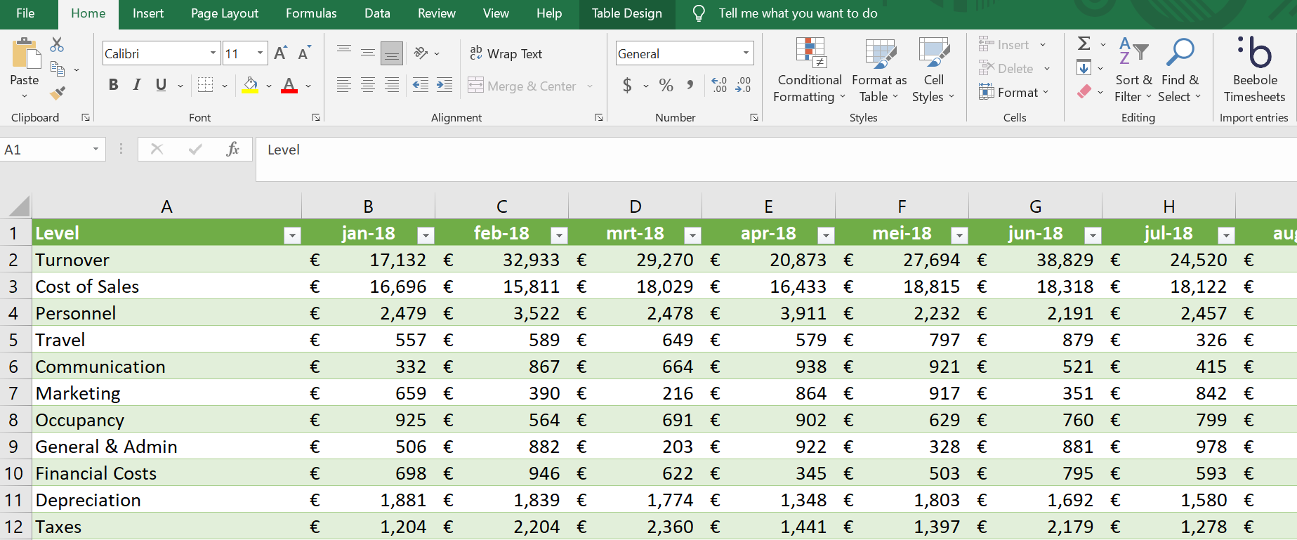

Table of Contents
Table of Contents
In this tutorial, learn how to create a budget vs. actuals report in Excel using Power Query. Gain insights and track financial performance effortlessly.
As a financial controller, accountant, or CFO, you’re likely familiar with the concept of budget vs. actuals. You know that reporting budget vs. actuals can be both cumbersome and time-consuming, given actuals are administered on a detailed level and budget numbers are recorded on a higher level. With this tutorial, however, we hope to show you it doesn’t need to be some cumbersome.
Managers are responsible for actual amounts spent versus the corresponding budgeted amounts per category. The actual amounts may be derived from the accounting system, while the budget amounts are retrieved from the official budget as determined and agreed upon at the end of last year for the current year. A budget is a report by cost/revenue category showing estimated numbers by month for the next year as agreed upon by management. The financial manager will report on these actual versus budget numbers, usually on a monthly basis and with a lot of manual effort. But using the built-in Power Query feature, the reporting procedure can be a breeze.
The key distinction between budget and actual expenditure is that the budget is a planned estimate of future financial activities, while actual expenditure represents the realized costs incurred in practice. The comparison between budgeted amounts and actual expenditures is crucial for evaluating financial performance, identifying variances, and making informed decisions to manage resources effectively. By analyzing these differences, organizations or individuals can assess their financial performance, adjust their future budgets, and take necessary corrective actions.
In summary, the key differences are:
By comparing budgeted amounts, forecasts, and actuals, individuals and organizations can assess their financial performance, identify variances, and make informed decisions to manage resources effectively.
Yes, budget vs. actuals analysis and budget to actual variance analysis are essentially the same thing. Both terms refer to the process of comparing budgeted amounts to actual results and analyzing the differences or variances between them.
Budget vs. actuals analysis involves assessing the financial performance by comparing the planned budgeted figures with the actual results that have been realized. It helps in evaluating how well the organization or individual has met their financial targets and objectives.
On the other hand, budget to actual variance analysis specifically focuses on identifying and analyzing the differences or variances between the budgeted amounts and the actual results. It involves calculating the variances for various income and expense categories, understanding the reasons behind the variances, and assessing their impact on the overall financial performance.
In both cases, the goal is to understand the variations between the planned budget and the actual outcomes, which can provide insights into areas of strength, areas needing improvement, and potential issues or opportunities for financial management and decision-making.
Therefore, while the terms may have slightly different wording, they generally refer to the same practice of comparing budgeted amounts to actual results and analyzing the variances to gain insights into financial performance. This analysis could also be part of a typical finance controller KPIs dashboard.
Creating a budget vs. actuals report can involve various labor-intensive steps when using Microsoft Excel the old-fashioned way. Luckily, however, modern Excel contains BI tools such as Excel Power Query and Power Pivot, which make creating a budget vs. actuals template much more attainable.
In this article, you will learn how to set up a dynamic model on budget vs. actuals in Excel using these tools. Apart from this being a painless process, rest assured you’ll end up with an accurate budget vs. actuals report that’s generated automatically. Let’s get started!
Having access to Microsoft Excel is a must. Then, be sure to download the file below to follow along with the tutorial.

Below, you’ll see screenshots for each of the tabs in the Excel file we’ll be working with. Those tabs are: Actual, Budget, Chart of Accounts, and Level.

This sheet is formatted as a table and is downloaded from an ERP system.

The budget numbers are recorded in a cross-table style, so it is easy to enter data as months go by. The user records the budget numbers at a higher level.

The Chart of Accounts shows all the accounts that can be used at an Actual level and the accompanying level for use in the Budget.

This table displays the levels and accompanying Order, Type, and Sign. The Order can be used to sort the final report in the desired order and sequence. The Type shows the type of account, i.e., BS (=Balance Sheet) and PL (Profit & Loss). Only Profit & Loss accounts will be presented in the final report. Sign can be used to transform detailed Actual amounts into the correct format. Debits and Credits will be shown as positive numbers.
In order to create a dynamic report, we need to go through the following 7 steps:
Place your cursor in the Actual table and select from the Ribbon: Data → Get & Transform Data → From Table/Range. A copy of your data will be placed in Power Query. To import the next table, you need to exit Power Query by selecting in the Ribbon: Home → Close → Close & Load → Close & Load to … → Only Create Connection → OK.

On the right-hand side, you will see a Queries & Connections Panel with the table just loaded.
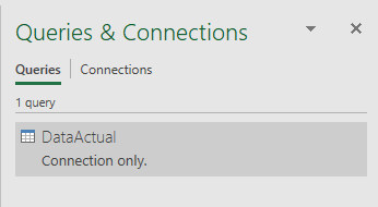
Now, move to the next tables and load them in the same fashion as the first table.
When you are done, you will see four queries appearing in the Queries & Connections Panel.
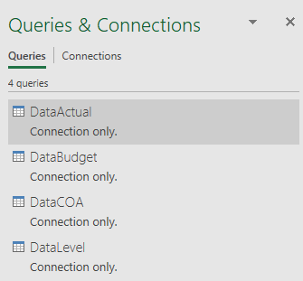
To transform the data, you need to return to the Power Query environment. You may do so by double-clicking on of the queries in the panel.
In Power Query, you can see all the queries by clicking on the >icon located on the left-hand side of the screen.

The Navigator Pane will open, and you’ll see the four queries.

We want to create a long table for DataBudget. Proceed as follows:
The Actuals are recorded at a detailed level, while the Budget is maintained at a higher level. To be able to connect to the Budget, you must convert Actuals to this higher level. To do so, select from the Ribbon: Home → Combine → Merge queries and select DataCOA as second table. Click on columns Acc No in both tables. You will notice that the selection matches, and a green check mark is displayed. Click on the OK button.

A new column will appear on the right-hand side. Click on the double arrow. Deselect all options in the dialog box, select Level, and click on the OK button.

Since revenues are booked as credit amounts, we want to revert them to positive numbers for reporting purposes. Furthermore, we only want to see Profit & Loss accounts. We need to merge the Actuals with Level and select from the Ribbon: Home → Combine → Merge queries and select DataLevel as second table. Click on columns Level in both tables. Notice that the selection matches and a green check mark appears. Click on the OK button.

A new column will appear on the right hand side. Click on the double arrow. Deselect all options in the dialog box, select Type and Sign, and click on the OK button.
Filter column Type on PL accounts by deselecting BS accounts.
Add a new column by selecting: Add column → Custom column. Enter the following details and click on OK.

Complete the transformation by performing the following steps:
In the Queries & Connections Panel you need to right-click on all the queries, and from the short menu, select: Load To… and then a dialogue box appears where you select: Add this data to the Data Model → OK.

When you are done, you will see in the Queries & Connections Panel that all the records for each query have been loaded into the Data Model.
To create relations between the tables, proceed as follows:

You need to create the following measures by selecting: Power Pivot → Calculations → Measures → New Measure:

In the same fashion, you will create the following measures:
Now we are ready to create a dynamic Pivot Table report. Select: Power Pivot → Data Model → Manage → Home → Pivot Table → Pivot Table → New worksheet → OK.

Use the following settings:
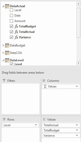
As you can see, the calculated measures are used as values, while DataLevel – Level is used to populate the rows.
In order to view the data by month, you can add a timeline. With your cursor placed in the pivot table, choose Pivot Table Analyze → Filter → Insert Timeline → Date → OK.

The dynamic Pivot Table, including the timeline, looks as follows:

By selecting the desired month, the accompanying numbers in the pivot table will change automatically.
By using the steps described in this article, you will create the actual vs. budget report in less time using just a few formulas. Once the source data is changed, you can simply update the report by choosing Data → Queries & Connections → Refresh All.
Project profitability analysis involves assessing the revenue, costs, and profit associated with a project to understand if it is financially beneficial. It primarily focuses on whether the project has or will achieve the desired return on investment.
On the other hand, budget versus actuals analysis is a method of comparing the budgeted costs of a project against the actual expenses incurred. This analysis helps in tracking the financial performance of a project, identifying variances, and implementing corrective actions.
The relationship between these two stems from their focus on project financials and performance. The results from a budget versus actuals analysis can significantly influence project profitability analysis: if actual costs are consistently over budget, it could indicate inefficiencies or unforeseen expenses, leading to lower profitability than initially projected. Conversely, if actual costs are consistently under budget without compromising the project’s output, it could indicate cost efficiency, potentially increasing the project’s profitability.
Therefore, effective budget versus actuals analysis can enable a more accurate project profitability analysis. It allows project managers to monitor costs, identify cost trends, and make necessary adjustments to ensure the project remains profitable. Similarly, project profitability analysis can offer valuable insights for refining the budgeting process, leading to more accurate and realistic budgets in the future.
If you’re a financial manager or someone who works with budgets and reporting regularly, we genuinely hope this tutorial shows that reporting budget vs actuals doesn’t need to be cumbersome or time-consuming.
–
Don’t miss our other tutorials on topics like Excel Power Query hacks and how to build an automated time tracking dashboard.
–
If you bill clients based on the time you spend, here’s a pop quiz: which projects make the most money? Or even more importantly: which projects aren’t profitable? If you don’t know the answer to these questions, it’s time to start thinking about project profitability, a measurement of revenue billed versus time and cost expended. […]
What is a payroll variance? Payroll variance is a running total of how much money your company has paid out to employees for things like overtime, vacation, sick days, and pay raises. It helps finance and HR managers figure out if budgets are being met and if everyone is getting paid the right amount. Payroll […]
If you’re remotely interested in project management, then you’ll likely be quite familiar with the scope-budget-time project management triangle. As with many tried-and-true ideas and theories, sometimes it can be good to hit refresh and come at it from a new angle. And that’s what I’d like to do today—let’s have a look at the […]
Thanks for the valuable tutorial. Is there anyway you can have these on video?
Hi Arthur!
Thanks so much for your comment, and thanks for reading. We are working on creating more content and tutorials on our YouTube page. You can check here: https://www.youtube.com/c/BeeBole
And more specifically, here is a playlist with various tutorials, and where we plan to add more soon: https://www.youtube.com/playlist?list=PL8xCZeiQjKb3PqtH1frf8py5kHpvpWFDf